IQ - Measuring Graph Intelligence

The Problem of Relative Complexity

“Cities are too complex” is not a statement of fact. It’s a refusal to specify what kind of complexity we mean. And it’s every statistician’s excuse for ignoring urban informatics.

ML researchers are only slightly better, but still routinely train models across cities as if they were exchangeable samples from a single data-generating process. This assumption is almost never stated, but infects our analyses: in graph embeddings trained jointly on Paris and Detroit, in navigation heuristics evaluated on Manhattan and Istanbul, in retrieval systems that treat “a city” as a homogeneous object.

Urban road networks are not generated by a single stochastic process. Paris is the partial output of centralized intervention (Haussmann). Istanbul is an accretion process constrained by topography, empire, and path dependence. Lagos, Prague, Manhattan—each reflects a distinct historical prior. Treating them as IID graph samples is not simplification; it is model misspecification.

Urbanists know that cities vary fundamentally based on location, scale, and culture. The non-obvious failure is that we lack a principled way to measure how they differ structurally, independent of geography, scale, or visual intuition.

So we ask a stronger question: If we strip a city of geometry and retain only adjacency—only topology, can we quantify the difference in structure between the local and the global?

This is a hypothesis, not a metaphor. And hypotheses deserve estimators and statistical inference.

Cities as Messages, Not Maps

Let a city’s road network be an undirected graph, denoted $G=(V,E)$, where $V$ is the node set and $E$ is the edge set.

An agent traversing this network does not experience the city globally. Even if it were given the global degree distribution, this may not be entirely sufficient for the complexity within the network itself. One such example is heterogeneity in degree distributions across subgraphs of the same city road network. It encounters induced subgraphs—local neighborhoods revealed incrementally. For any subset $S \subseteq V$, let $G[S]$ denote the induced subgraph.

We treat each $G[S]$ as a finite message describing local structure. Vitanyi et al. then give us a strong basis for quantifying the information content of such a message as an indicator of representational complexity.

How many bits are required to describe this subgraph, and how does that compare to what we would expect if the city were structurally uniform?

This reframes network information as a coding problem. And this is something that we can test.

The Null: Erdős–Rényi as a (Simple) Universal Baseline

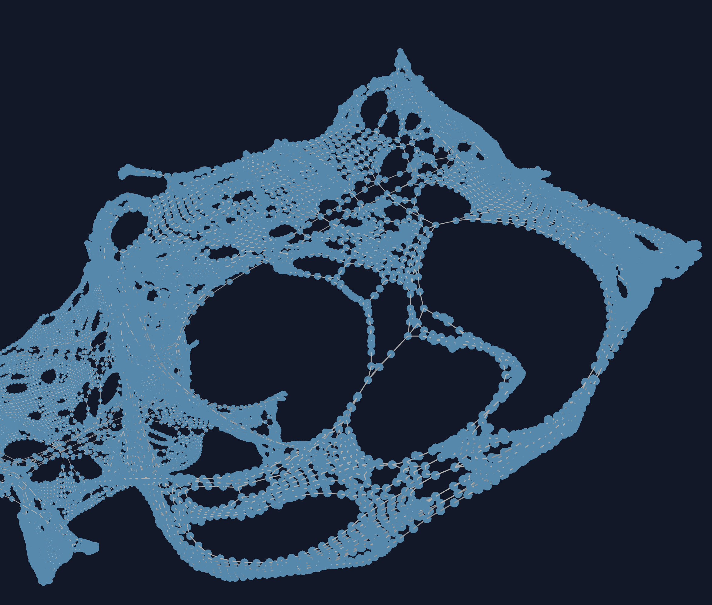
We need a reference model. This defines what we consider to be a “random” state under our null hypothesis. Put simply: if we want to tell whether a fuzzy image depicts a cat, we’ll probably need to compare it with other images we know to be cats. Against this assumption that a cat has certain features defined by our null model (ears, fur, (usually) 4 legs), how much does this fuzzy picture align with our expectations?

For a subgraph with $n = |S|$, $m = |E(G[S])|$, and $M_S = \binom{n}{2}$, we assume an Erdős–Rényi model $G(n,p)$, where edges occur independently with probability $p$.

Under this model: $P(G[S] \mid p) = p^m (1-p)^{M_S - m}.$ This means that the probability of any particular arrangement of roads and intersections is distributed according to this model, which is described by a single parameter $p$.

Using base-2 logarithms throughout (so description lengths are in bits), the corresponding Shannon code length is: $L(G[S] \mid p) = -\left[m \log_2 p + (M_S - m)\log_2(1-p)\right].$

ER is the maximum entropy model subject to a single constraint (edge density). Any deviation from it must be explained by some presence of structure. And the higher the subgraph differs from the global baseline, the stronger an indication of structure to our network.

Methods (at a Glance)

We include a rough outline of the methods used to re-create the analysis.

Constructing the Local Subgraph

• For seed node $v \in V$ and radius $r$, define the ego subgraph $G_r(v)=G[\{u:d(u,v)\le r\}].$
• For each local subgraph, compute the nodes, edges, and likelihood:
  • $n=|S|$
  • $m=|E(G[S])|$
  • $M_S=\binom{n}{2}$

Computing our Null Hypothesis.

• Use an Erdős–Rényi baseline $G(n,p)$ with edge probability $p$.
• We convert the divergence to bits by using the log-2 operation: $L(G[S]\mid p)=-\left[m\log_2 p+(M_S-m)\log_2(1-p)\right].$

Computing the Divergence Between Local and Global Densities.

• Let $p_{\text{global}}$ be the global edge-density baseline and $p_{\text{local}}=m/M_S$ the local fit.
• Define penalized divergence as $\Delta L_{\text{ER}}(G[S])=L(G[S]\mid p_{\text{global}})-\Big[L(G[S]\mid p_{\text{local}})+\tfrac12\log_2 M_S\Big].$
• We report normalized variants (e.g., per potential edge) when comparing across radii/cities.

Generating IQ Profiles over Iterative Traversals.

• We use the same ER MDL measurements defined in the Introduction, $\mathrm{IQ}(r)=\mathbb{E}\!\left[\frac{1}{M_r}\,\Delta L_{\text{ER}}(G_r(v))\right],$ where expectation is approximated by random seed-node sampling.

Validating the Divergence Measure on Synthetic Networks.

• Before testing on road networks, we validate the measure on simulated networks of known models. This is to make sure it can detect the various kinds of structure that distinguish network models.
• To compute uncertainty measurements, we perform node subsampling over a series ($n=500$) of seed nodes. This also alleviates the issue of working with a single possible city network: it becomes difficult to run simulations of multiple trials.

Absolute vs. Relative Description Length

A dense subgraph is not necessarily complex. Density is not structure. We have to distinguish between the two, and we do this by computing not one estimate of minimum description length, but two.

The “baseline” is the divergence of the model when fit to the entire network. We call this the global baseline because it describes the network when considered as a whole.

We contrast this with an MDL estimate that is specifically local in scope, called our local intervention. The local minimum description length is that of a model when fit to an induced ego-graph

What do we mean by local versus global complexity?Show

Naively, the local model always fits better since it is optimized for that particular subgraph. And to encode the length of the model parameters itself, we add a normalization term. This penalizes the model for its complexity—every additional parameter incurs a cost. This ensures the model doesn’t simply fit to the exact subgraph.

Using the standard stochastic complexity with a penalty for model description length (one parameter, sample size $M_S$): $L_{\text{local}}(G[S]) \approx -\log_2 P(G[S]\mid p_{\text{local}}) + \tfrac{1}{2}\log_2 M_S.$

And then we have everything we need to create a normalized estimator. Not only does it involve the model description length, but ensure the model doesn’t encode the observed dataset in its entirety. The penalized MDL divergence is then:

$\Delta L_{\text{ER}}(G[S]) = L(G[S]\mid p_{\text{global}}) - \Big[ L(G[S]\mid p_{\text{local}}) + \tfrac{1}{2}\log_2 M_S \Big].$

Interpretation: Not only are we interested in the pure MDL of the network (whose minimal absolute description encodes the entire network), but an MDL measure that penalizes the complexity of our model.

What do we mean by 'penalizing' model complexity?Show

Asymptotically, $\frac{1}{M_S}\Delta L_{\text{ER}} \approx D_{\mathrm{KL}}\big( \text{Bern}(p_{\text{local}}) || \text{Bern}(p_{\text{global}})\big),$ up to finite-sample correction.

This estimator calculates well the amount of structure that exists beyond pure chance of degree-connectivity.

Traversal, Not Snapshots: The IQ Profile

Complexity is scale-dependent. A cul-de-sac looks simple until it opens into a maze.

For a root node v, define the radius-r ego graph: $G_r(v) = G[\{u : d(u,v)\le r\}]$.

We define the Local Complexity Profile (IQ) as: $\mathrm{IQ}(r) = \mathbb{E}\!\left[ \frac{1}{M_r}\, \Delta L_{\text{ER}}(G_r(v)) \right],$ where expectation is taken over randomly sampled seed nodes.

As $r \to \infty$, this profile is expected to approach zero as the local view approaches the full city graph. The rate of convergence is the signal of interest.

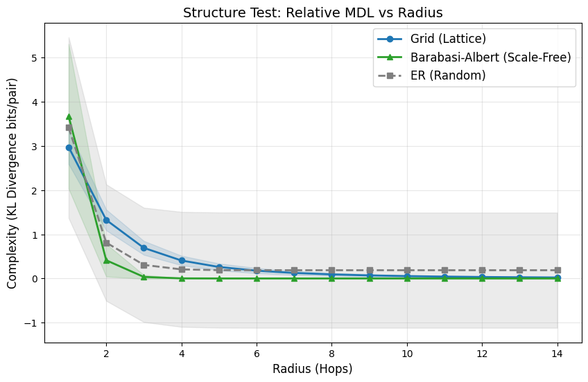
We validate the estimator against synthetic families:

• Grids: slow convergence—loops must be “learned.”
• Scale-free networks: rapid convergence—hubs expose global structure quickly.
• Erdős–Rényi graphs: no convergence to zero—residual randomness persists.

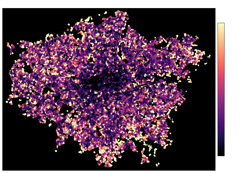
How this Shows Up on Actual Maps

When applied to actual road networks, the distinction is visually distinguishable even in the complexity profile.

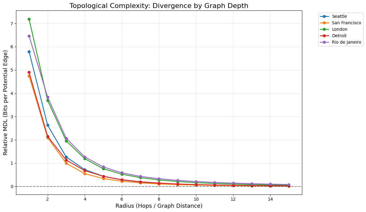
These behaviors are not cosmetic. They correspond exactly to the traversal experience of an agent with limited horizon. And the Erdős–Rényi test was one of our strongest validations. When we control for a stable amount of randomness, we intentionally create noise that the measure cannot compress. This appears on the MDL curves as a line that hovers just above zero.

Even applied to real cities, the ordering is stable. London’s IQ dominates Detroit’s and San Francisco’s at nearly all radii. Manhattan collapses quickly. Lagos exhibits persistent divergence. These results survive node subsampling (à la Lunde) resampling, seed variation, and traversal depth.

Crucially, the measure ignores geometry entirely.

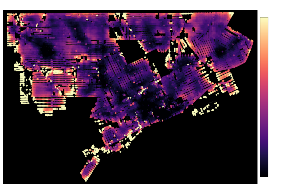
Downtown Detroit looks visually chaotic because of highway intrusions and the radial layout of historically French boulevards. Yet the measure ignores the radial curve of the streets to reduce the dense streets to exactly what they are: a simple lattice. This suggests that the measure distinguishes well between geometry of the network and its substructures.

London, on the other hand, remains structurally surprising at nearly every scale. There is a persistent heterogeneity in the city’s road networks, indicating frequent divergence from the global norm. There is rarely a point while traversing London’s road network where an agent has sufficient information about the whole. Such a network can justifiably be considered more complex.

Complexity, in this sense, is not subjective. But our intuitions about it often are. We’re influenced by visual density and the irregularities that we can discern from a glance. The estimator is stronger in that it assigns an appropriate quantity structural differences both seen and unseen to the eyes of a human.

Why This Matters

Most ML systems on cities quietly assume structural stationarity. Our results demonstrate quantitatively that this assumption fails within cities, not just between them.

One critique worth surfacing explicitly: ER is a blunt null. Degree-corrected or configuration-model baselines would isolate higher-order motifs more cleanly. We’re working on expanding the metric for other reference models to describe complexity at a finer grain.

But as a first-principles estimator of relative structural surprise under traversal, the construction is sound, falsifiable, and empirically testable…so we’re doing better than most network scientists. (for the sake of preserving collaborations: we joke!)

We did this work because we’re increasingly opposed to the claim that cities are “too complex” by their very nature. They are differentially informative, which is to say that every neighborhood and street corner can still teach us something new.

And information, at least, we know how to measure.