Local MDL-Based Divergence for Structural Complexity Analysis
Abstract
In this work, we introduce a localized, MDL-based divergence measure that quantifies the structural complexity of induced subgraphs relative to a global reference model. The measure compares the compressibility of local neighborhoods under globally fitted and locally optimized comparator models while penalizing model flexibility, yielding a statistically grounded notion of local structural surprise. The results show that the measure converges under controlled ablations, is robust to sampling choices, and detects meaningful structural irregularities that are invariant to geometric embedding. This framework generalizes MDL-based network analysis to arbitrary information graphs and provides a principled bridge between global structure and agent-level experience.
Cite this work
Show citation formats
Kennon Stewart (2026). Local MDL-Based Divergence for Structural Complexity Analysis.@inproceedings{mdl_divergence_2026,
title={Local MDL-Based Divergence for Structural Complexity Analysis},
author={Kennon Stewart},
year={2026},
}Introduction
Graphs are an elegant means to model structured information. They encode relationships within systems as diverse as cities, biological systems, and causal relationships. In nearly all of these contexts, however, graphs are not encountered as complete objects. They are traversed locally by agents, human or otherwise, who observe only a bounded neighborhood at any given step and must act under uncertainty about the larger structure.
Despite this, most of network science focuses on global structures. Statistical and generative network models are designed to summarize entire graphs using aggregate statistics and likelihoods. These methods are well suited for comparing networks at scale, but they implicitly assume a homogeneous network with no sense of emergent complexity.
This assumption is increasingly misaligned with how graphs are used. In navigation, reasoning, search, and planning tasks, agents experience networks in episodes determined by a sequence of traversal decisions. What matters is not whether the graph is globally regular or compressible, but whether the next few steps are predictable given what has already been observed. Two graphs with identical global statistics may pose radically different local decision problems, while visually complex structures may be informationally sparse once reduced to their relational form.
To formalize this idea, we introduce a localized MDL-based divergence measure. For a given induced subgraph, we compare its description length under a globally fitted reference model to that under a locally optimized model. While doing so, we penalize the latter for its complexity to prevent overfitting. This construction ensures that apparent irregularities are only credited when they exceed what can be explained by chance, sparsity, or small sample effects. In the large-sample limit, the measure converges to a Kullback-Leibler divergence between local and global statistics, grounding it in classical information theory.
By shifting the focus from global summaries to local experience, this work extends MDL-based network analysis to settings where agents reason, navigate, or infer under partial information. The framework is intended not as a replacement for global complexity measures, but as a complementary tool for understanding how structure manifests at the scale where decisions are actually made.
Contribution
We introduce a general, agent-centric definition of local complexity for networks. Local complexity is formalized as relative incompressibility: the extent to which a subgraph resists encoding under a global reference model. This reframing decouples complexity from geometry and global summary statistics.
Related Work
Kolmogorov Complexity and the Minimum Description Length Principle
The assessment of information density in complex systems is fundamentally divided between information-theoretic measures of uncertainty and structure-theoretic measures of regularity. Shannon entropy provides the foundational information-theoretic limit, defining the expected optimal coding rate for symbols drawn from a known probability distribution. However, because Shannon’s theory assumes the distribution is given, it effectively treats learnable statistical information as zero and measures only the uncertainty of the message. For structural analysis, Kolmogorov complexity is used instead, which defines an object’s absolute information content as the length of the shortest binary program required to perfectly reproduce it [li_introduction_2008].
Because is not directly computable, the Minimum Description Length principle serves as a practical implementation of Occam’s Razor. This reframes learning as a data compression problem where the best model is the one that achieves the shortest total description. This framework typically employs a two-part code that decomposes total information into two components: the complexity of the model, indicating regular features, and the entropy of the data given the model, indicating unexplained variance.
More recent work in complex systems analysis notes that classical MDL assumes standard models where the Fisher information matrix is non-singular and complexity grows linearly with parameter count. However, many complex systems are singular models where multiple sufficient states satisfy performance constraints.
In such systems, the Local Learning Coefficient is a more accurate measure of complexity than parameter counting. It accounts for the volume of the loss landscape and the effective dimension of the model [Lau_Furman_Wang_Murfet_Wei_2024]. High compressibility in these systems indicates a lower learning coefficient, suggesting that the system has discovered a general solution rather than merely memorizing the training data.
Statistical Network Theory
Networks are a general structure for modeling the relationships between discrete states. They have been used to model social networks [Andris_2021], community resilience [Kim_Chung_Lee_2019], and the impact of social development projects [Lienert_Schnetzer_Ingold_2013], proving foundational to urban science. These methods use network-structured data for mapping social and organizational connections, which are typically underexplored in network theory research.
The field of network modeling is primarily divided into generative and feature-driven statistical methods, which provide distinct ways of understanding graph topology. The primary difference between the two is their focus: a generative network is formed through a series of local network rules, while statistical methods constrain the model in its global structure. This difference is fundamental and illustrates a broader divide in the analysis of mesoscale structure within networks.
Statistical Network Models
Statistical models are used to quantitatively describe the likelihood of an observed network by fitting parameters. These models, such as the stochastic block model, assume that nodes within the same group are statistically indistinguishable, allowing the global topology to be represented as a set of aggregate building blocks. In this framework, an induced subgraph is treated as a finite message, and its complexity is measured by the length of the shortest description required to encode it.
Under a baseline Erdos-Renyi assumption [Newman_2018], where each edge appears independently with probability , the probability of observing a particular graph is . The corresponding Shannon code length is the negative log-likelihood:
Statistical models enable formal inference by way of method of moments, maximum likelihood estimation, or Bayesian inference, where parameters are tuned to minimize the total description length.
Generative Network Models
Generative models specify a data-generating procedure or a sequence of local rules to explain the emergence of qualitative graph patterns. Unlike static statistical models, these are often growth models that iteratively add nodes and edges, such as the Barabasi-Albert model, which uses the preferential attachment principle to explain power-law degree distributions.
Other generative mechanisms include the copying principle, where new nodes duplicate the edges of existing nodes with some mutations, and recursion-based algorithms like R-MAT that generate self-similar hierarchical structures. These models facilitate the study of network evolution and allow researchers to simulate realistic synthetic datasets that capture empirical properties like the small-world effect or shrinking diameters.
These two principles converge in the MDL framework, which decomposes a network’s description into two parts:
This approach ensures that a model is only considered a better explanation for the data if the compression gain it provides outweighs the information cost of describing its parameters. By calculating the relative MDL divergence between a local subgraph and a global null model, researchers can identify structural irregularities that are topologically invariant and quantify the epistemic effort required to traverse the network.
Methods
Graphs as Messages
Let be an undirected graph with nodes and edges. For any subset , denote by the induced subgraph on .
We treat each induced subgraph as a finite message describing the local structure encountered by an agent traversing the network. This means quantifying local structural complexity relative to a reference model. While methods like Bayesian stochastic block modeling quantify the network’s global complexity [peixoto_bayesian_2023], the emergent complexity of the network at increasing scales remains underspecified.
Erdos-Renyi Comparator
The single-parameter comparator is the Erdos-Renyi model. It assumes a global edge probability such that the probability of any particular arrangement of edges in a network of nodes follows a binomial law. We define:
Under , the probability of observing a particular graph with edges is
The corresponding Shannon code length is the negative log-likelihood of the model:
The stochastic complexity of the subgraph adds a penalty for model flexibility to encourage regularization [Myung_Navarro_Pitt_2006]. Using the standard Fisher information approximation, the code length for the local model is:
Here, the penalty term represents the number of bits required to encode the parameter itself, where and the sample size is .
Absolute versus Relative Complexities
We fit two Erdos-Renyi models: one fit to the local density and the other fit to the global density . This design choice allows for a balanced comparison between sparse and dense networks. Normalizing by the total number of potential edges accounts for the fact that both the presence and absence of an edge are relevant to the encoding.
The penalized MDL divergence is then defined as the savings achieved by the local model after the penalty:
For large samples, the measure converges to the Kullback-Leibler divergence:
Local structural complexity is thus the KL divergence between local and global statistics, while filtering for significance. If the divergence is small, meaning the neighborhood looks roughly like the average city street, the penalty term dominates and drives to zero or below. Positive values indicate true structural anomalies that cannot be explained by chance or small-sample noise.
Results
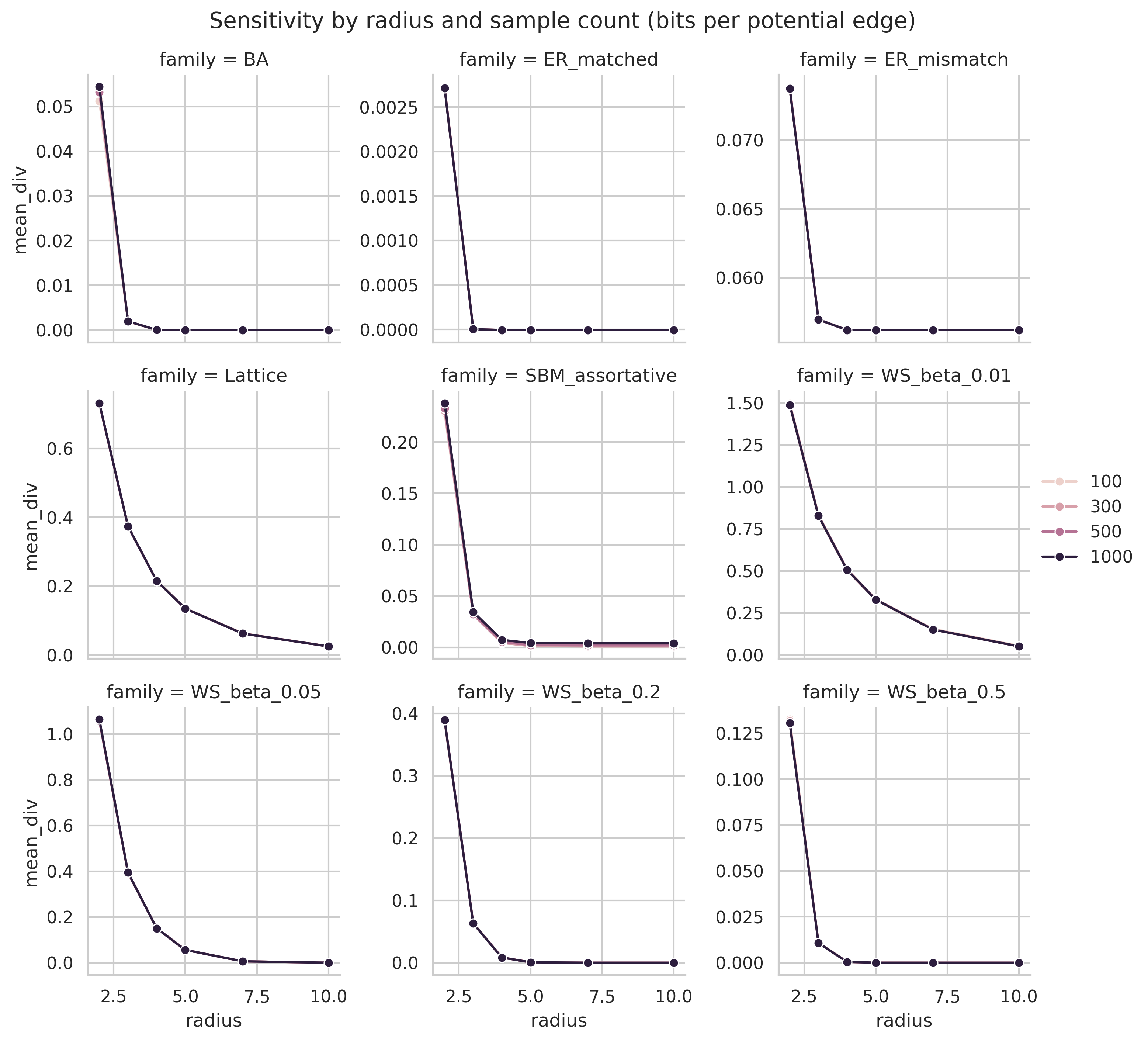
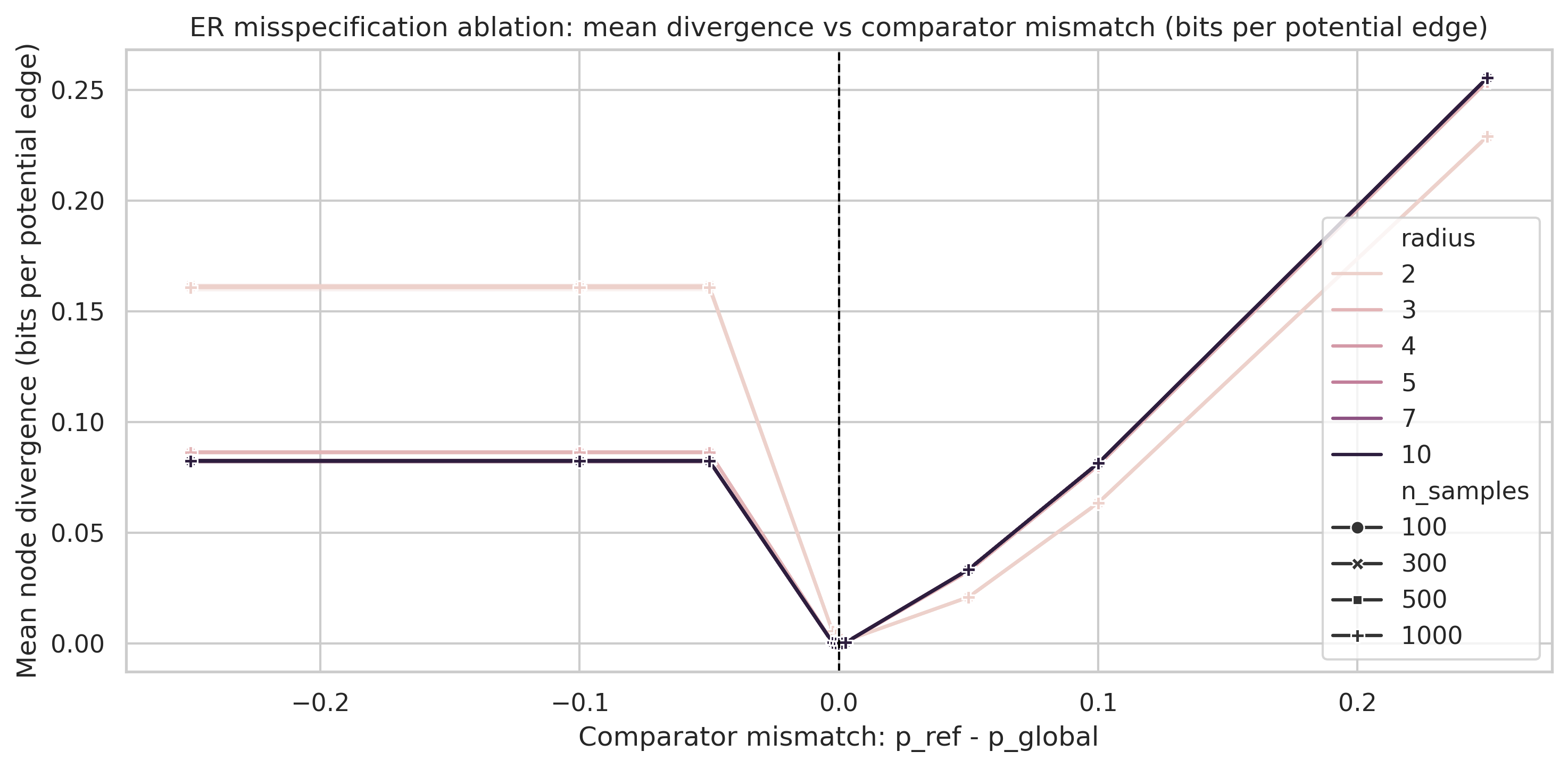
Results empirically show that MDL divergence distinguishes model families. Under the degree-matched ER null, the profile peaks early and then collapses to negative values at large radii. This empirically supports the theoretical convergence of local substructure toward the global profile. Model families for which the structural mismatch persists show a much higher asymptotic divergence than those whose irregularities are transient.
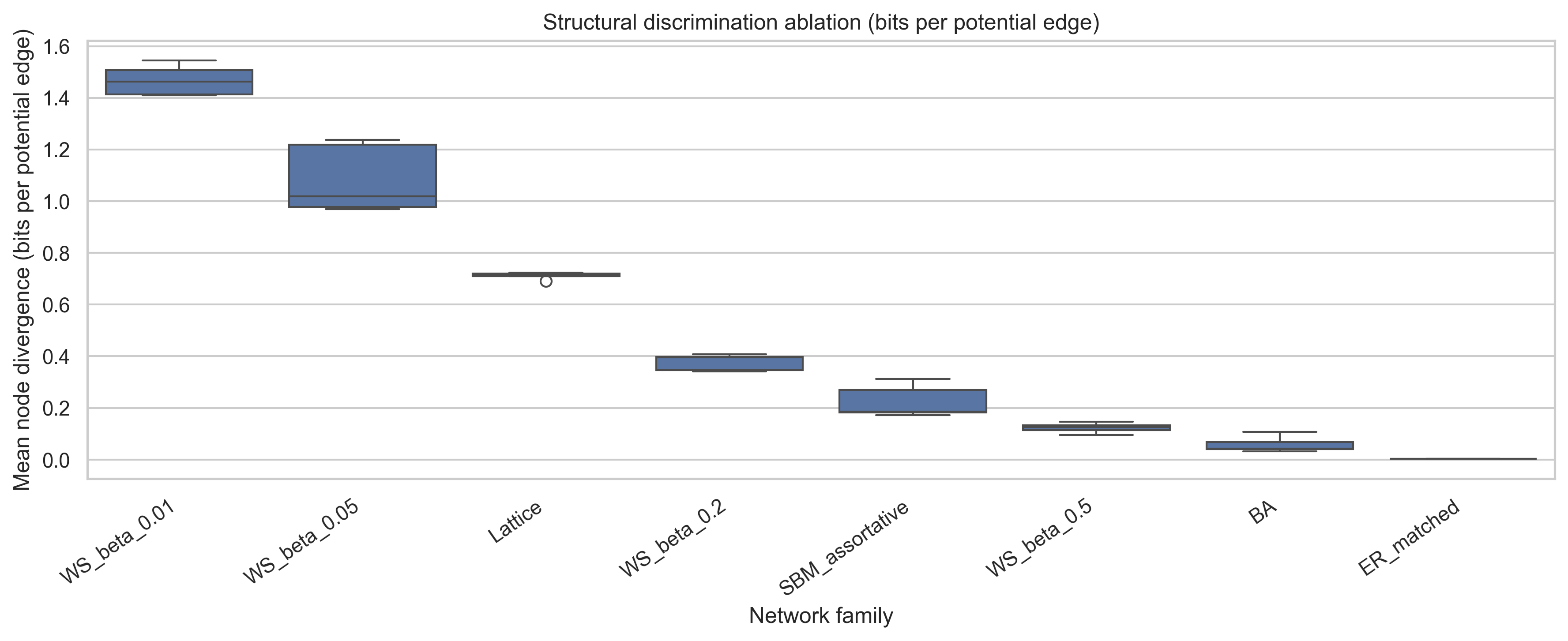
The families also separate by the scale at which irregularity appears. Barabasi-Albert, SBM, and the more highly rewired Watts-Strogatz model peak at small radii and then decay toward zero. By contrast, lattice and low- ablations continue to accumulate positive normalized signal out to the largest tested radius. That distinction shows that the normalized statistic distinguishes persistent irregularity from transient mesoscale structure.
Ablation results for normalized localized MDL divergence on synthetic graph families with known structural irregularities.
| Family | AUC | Peak Radius | Peak Divergence |
|---|---|---|---|
| ER matched | 253.6 [235.1, 274.0] | 3 | 129.6 [125.3, 134.3] |
| ER mismatch | 1655.5 [1618.1, 1697.1] | 4 | 484.1 [464.6, 507.1] |
| Lattice | 1905.8 [1902.5, 1910.0] | 10 | 380.9 [380.2, 381.8] |
| WS beta = 0.01 | 3011.5 [2907.0, 3086.5] | 10 | 563.6 [546.3, 578.0] |
| WS beta = 0.05 | 2290.7 [2168.5, 2504.6] | 6 | 453.5 [441.4, 468.7] |
| WS beta = 0.2 | 734.8 [697.2, 768.6] | 4 | 270.0 [259.3, 277.9] |
| SBM | 435.7 [410.8, 461.4] | 4 | 161.8 [154.7, 168.4] |
| Barabasi-Albert | 371.3 [354.4, 387.8] | 3 | 204.3 [187.3, 224.9] |
The table separates families along two distinct axes: total accumulated irregularity and the radius at which that irregularity is most pronounced. High-AUC families sustain mismatch over many scales, whereas earlier peak radii indicate irregularity that is more localized and decays quickly.
The resulting qualitative ordering is also more interpretable with respect to the corresponding network family. Weakly rewired Watts-Strogatz graphs, lattice-like graphs, and comparator misspecification sustain the largest cumulative normalized divergence. Barabasi-Albert and SBM produce earlier, more localized peaks. The matched ER family has the smallest cumulative signal and ends in the penalty-dominated regime. That is the contrast one would want in an ablation section built around known structural irregularities.
References
- Ming Li, P. M. B. Vitanyi (2008). An introduction to Kolmogorov complexity and its applications. Texts in Computer Science. Springer.
- Edmund Lau, Zach Furman, George Wang, Daniel Murfet, Susan Wei (2024). The Local Learning Coefficient: A Singularity-Aware Complexity Measure. arXiv. arXiv. https://doi.org/10.48550/arXiv.2308.12108
- Clio Andris, Xi Liu, Jessica Mitchell, James O'Dwyer, Jeremy Van Cleve (2021). Threads across the urban fabric: Youth mentorship relationships as neighborhood bridges. Journal of Urban Affairs. Routledge. https://doi.org/10.1080/07352166.2019.1662726
- Hwanbae Kim, Jae-Kyoung Chung, Myeong-Hun Lee (2019). Social Network Analysis of the Jangwi Urban Regeneration Community. Sustainability. MDPI AG. https://doi.org/10.3390/su11154185
- Judit Lienert, Florian Schnetzer, Karin Ingold (2013). Stakeholder analysis combined with social network analysis provides fine-grained insights into water infrastructure planning processes. Journal of Environmental Management. Elsevier. https://doi.org/10.1016/j.jenvman.2013.03.052
- Mark Newman (2018). Networks. Oxford University Press. https://doi.org/10.1093/oso/9780198805090.001.0001
- Tiago P. Peixoto (2023). Bayesian stochastic blockmodeling. arXiv. arXiv. https://doi.org/10.48550/arXiv.1705.10225